Reading and Writing Equations Using One Variable

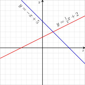
Equation that does not involve powers or products of variables

Two graphs of linear equations in two variables

In mathematics, a linear equation is an equation that may be put in the form

a_{1}x_{1}+\cdots +a_{n}x_{n}+b=0,

where $x_{1},\ldots ,x_{north}$ are the variables (or unknowns), and $b,a_{1},\ldots ,a_{n}$ are the coefficients, which are often real numbers. The coefficients may be considered as parameters of the equation, and may exist arbitrary expressions, provided they practise not comprise whatever of the variables. To yield a meaningful equation, the coefficients $a_{one},\ldots ,a_{n}$ are required to not all be zero.

Alternatively a linear equation can be obtained past equating to zero a linear polynomial over some field, from which the coefficients are taken.

The solutions of such an equation are the values that, when substituted for the unknowns, brand the equality true.

In the case of only one variable, at that place is exactly one solution (provided that $a_{i}\neq 0$ ). Often, the term linear equation refers implicitly to this particular case, in which the variable is sensibly called the unknown.

In the case of two variables, each solution may be interpreted as the Cartesian coordinates of a betoken of the Euclidean plane. The solutions of a linear equation class a line in the Euclidean plane, and, conversely, every line can be viewed as the set of all solutions of a linear equation in ii variables. This is the origin of the term linear for describing this type of equations. More more often than not, the solutions of a linear equation in $n$ variables form a hyperplane (a subspace of dimension $n - 1$ ) in the Euclidean infinite of dimension $due north$ .

Linear equations occur frequently in all mathematics and their applications in physics and engineering science, partly considering non-linear systems are often well approximated by linear equations.

This commodity considers the case of a single equation with coefficients from the field of real numbers, for which one studies the existent solutions. All of its content applies to circuitous solutions and, more more often than not, for linear equations with coefficients and solutions in any field. For the case of several simultaneous linear equations, see organisation of linear equations.

I variable [edit]

Oftentimes the term linear equation refers implicitly to the example of just ane variable.

In this case, the equation tin be put in the course

ax+b=0,

and it has a unique solution

x=-{\frac {b}{a}}

in the full general case where $a \neq 0$ . In this example, the name unknown is sensibly given to the variable $x$ .

If $a = 0$ , there are two cases. Either $b$ equals also 0, and every number is a solution. Otherwise $b \neq 0$ , and there is no solution. In this latter case, the equation is said to exist inconsistent.

Ii variables [edit]

In the case of two variables, any linear equation tin exist put in the form

ax+by+c=0,

where the variables are $x$ and $y$ , and the coefficients are $a$ , $b$ and $c$ .

An equivalent equation (that is an equation with exactly the same solutions) is

Ax+Past=C,

with $A = a, B = b$ , and $C = - c$

These equivalent variants are sometimes given generic names, such equally full general form or standard course.^[1]

There are other forms for a linear equation (see below), which can all exist transformed in the standard form with unproblematic algebraic manipulations, such as calculation the same quantity to both members of the equation, or multiplying both members past the same nonzero constant.

Linear function [edit]

If $b \neq 0$ , the equation

ax+by+c=0

is a linear equation in the single variable $y$ for every value of $x$ . It has therefore a unique solution for $y$ , which is given by

y=-{\frac {a}{b}}x-{\frac {c}{b}}.

This defines a function. The graph of this function is a line with slope $-{\frac {a}{b}}$ and $y$ -intercept $-{\frac {c}{b}}.$ The functions whose graph is a line are generally called linear functions in the context of calculus. Yet, in linear algebra, a linear function is a function that maps a sum to the sum of the images of the summands. And so, for this definition, the to a higher place function is linear but when $c = 0$ , that is when the line passes through the origin. For avoiding confusion, the functions whose graph is an capricious line are often called affine functions.

Geometric interpretation [edit]

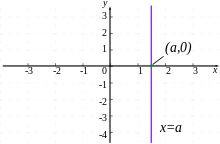
Vertical line of equation $10 = a$

Horizontal line of equation $y = b$

Each solution $(x, y)$ of a linear equation

ax+by+c=0

may be viewed equally the Cartesian coordinates of a point in the Euclidean plane. With this interpretation, all solutions of the equation form a line, provided that $a$ and $b$ are not both zippo. Conversely, every line is the set of all solutions of a linear equation.

The phrase "linear equation" takes its origin in this correspondence between lines and equations: a linear equation in two variables is an equation whose solutions form a line.

If $b \neq 0$ , the line is the graph of the office of $x$ that has been defined in the preceding section. If $b = 0$ , the line is a vertical line (that is a line parallel to the $y$ -axis) of equation $x=-{\frac {c}{a}},$ which is not the graph of a role of $x$ .

Similarly, if $a \neq 0$ , the line is the graph of a function of $y$ , and, if $a = 0$ , ane has a horizontal line of equation $y=-{\frac {c}{b}}.$

Equation of a line [edit]

There are diverse ways of defining a line. In the post-obit subsections, a linear equation of the line is given in each case.

Slope–intercept form or Slope-intercept form [edit]

A non-vertical line can exist divers by its slope $m$ , and its $y$ -intercept $y 0$ (the $y$ coordinate of its intersection with the $y$ -axis). In this case its linear equation tin be written

y=mx+y_{0}.

If, moreover, the line is not horizontal, information technology can exist defined by its slope and its $x$ -intercept $100$ . In this case, its equation can be written

y=thousand(ten-x_{0}),

or, equivalently,

y=mx-mx_{0}.

These forms rely on the habit of considering a non vertical line as the graph of a part.^[two] For a line given by an equation

ax+by+c=0,

these forms tin can be easily deduced from the relations

{\begin{aligned}m&=-{\frac {a}{b}},\\x_{0}&=-{\frac {c}{a}},\\y_{0}&=-{\frac {c}{b}}.\end{aligned}}

Point–slope grade or Point-gradient grade [edit]

A non-vertical line tin be defined by its gradient $one thousand$ , and the coordinates $x_{i},y_{1}$ of any point of the line. In this case, a linear equation of the line is

y=y_{i}+m(x-x_{i}),

y=mx+y_{1}-mx_{1}.

This equation tin can also be written

y-y_{1}=chiliad(10-x_{i})

for emphasizing that the slope of a line tin can be computed from the coordinates of whatsoever two points.

Intercept form [edit]

A line that is not parallel to an axis and does not pass through the origin cuts the axes in two dissimilar points. The intercept values $x 0$ and $y 0$ of these two points are nonzero, and an equation of the line is^[3]

{\frac {x}{x_{0}}}+{\frac {y}{y_{0}}}=1.

(Information technology is easy to verify that the line divers by this equation has $x 0$ and $y 0$ as intercept values).

2-point grade [edit]

Given two different points $(x 1, y ane)$ and $(10 ii, y two)$ , there is exactly one line that passes through them. At that place are several means to write a linear equation of this line.

If $x ane \neq x 2$ , the slope of the line is ${\frac {y_{two}-y_{1}}{x_{two}-x_{one}}}.$ Thus, a point-slope form is^[3]

y-y_{i}={\frac {y_{2}-y_{i}}{x_{two}-x_{ane}}}(x-x_{i}).

By immigration denominators, one gets the equation

(x_{2}-x_{1})(y-y_{1})-(y_{2}-y_{i})(ten-x_{ane})=0,

which is valid likewise when $10 i = x 2$ (for verifying this, it suffices to verify that the two given points satisfy the equation).

This form is not symmetric in the two given points, just a symmetric form tin be obtained past regrouping the constant terms:

(y_{i}-y_{two})x+(x_{two}-x_{1})y+(x_{1}y_{2}-x_{2}y_{i})=0

(exchanging the two points changes the sign of the left-hand side of the equation).

Determinant form [edit]

The 2-point form of the equation of a line can exist expressed simply in terms of a determinant. In that location are ii common ways for that.

The equation $(x_{ii}-x_{1})(y-y_{1})-(y_{2}-y_{one})(ten-x_{one})=0$ is the result of expanding the determinant in the equation

{\begin{vmatrix}10-x_{one}&y-y_{1}\\x_{2}-x_{1}&y_{2}-y_{1}\end{vmatrix}}=0.

The equation $(y_{one}-y_{ii})10+(x_{2}-x_{1})y+(x_{1}y_{2}-x_{two}y_{1})=0$ tin exist obtained be expanding with respect to its first row the determinant in the equation

{\brainstorm{vmatrix}x&y&1\\x_{i}&y_{1}&1\\x_{2}&y_{2}&1\finish{vmatrix}}=0.

Beside beingness very simple and mnemonic, this grade has the advantage of being a special case of the more general equation of a hyperplane passing through $n$ points in a space of dimension $due north - 1$ . These equations rely on the condition of linear dependence of points in a projective space.

More than than two variables [edit]

A linear equation with more than two variables may always be causeless to have the form

a_{1}x_{1}+a_{two}x_{2}+\cdots +a_{due north}x_{n}+b=0.

The coefficient $b$ , often denoted $a 0$ is called the constant term (sometimes the absolute term in old books^[4] ^[v]). Depending on the context, the term coefficient can be reserved for the $a i$ with $i > 0$ .

When dealing with $n=3$ variables, it is common to use $x,\;y$ and $z$ instead of indexed variables.

A solution of such an equation is a $n$ -tuples such that substituting each chemical element of the tuple for the corresponding variable transforms the equation into a true equality.

For an equation to be meaningful, the coefficient of at least one variable must exist not-zero. In fact, if every variable has a goose egg coefficient, then, as mentioned for one variable, the equation is either inconsistent (for $b \neq 0$ ) every bit having no solution, or all $due north$ -tuples are solutions.

The $n$ -tuples that are solutions of a linear equation in $n$ variables are the Cartesian coordinates of the points of an $(n - 1)$ -dimensional hyperplane in an $n$ -dimensional Euclidean space (or affine space if the coefficients are complex numbers or belong to whatsoever field). In the case of three variable, this hyperplane is a aeroplane.

If a linear equation is given with $a j \neq 0$ , and so the equation can be solved for $x j$ , yielding

x_{j}=-{\frac {b}{a_{j}}}-\sum _{i\in \{1,\ldots ,northward\},i\neq j}{\frac {a_{i}}{a_{j}}}x_{i}.

If the coefficients are real numbers, this defines a real-valued function of $n$ real variables.

Run into also [edit]

Linear equation over a ring
Algebraic equation
Linear inequality

Notes [edit]

^ Barnett, Ziegler & Byleen 2008, pg. fifteen
^ Larson & Hostetler 2007, p. 25
^ ^a ^b Wilson & Tracey 1925, pp. 52-53
^ Charles Hiram Chapman (1892). An Unproblematic Course in Theory of Equations. J. Wiley & sons. p. 17. Extract of page 17
^ David Martin Sensenig (1890). Numbers Universalized: An Advanced Algebra. American Book Visitor. p. 113. Excerpt of page 113

References [edit]

Barnett, R.A.; Ziegler, K.R.; Byleen, G.E. (2008), College Mathematics for Business, Economics, Life Sciences and the Social Sciences (11th ed.), Upper Saddle River, N.J.: Pearson, ISBN978-0-13-157225-6
Larson, Ron; Hostetler, Robert (2007), Precalculus:A Curtailed Course , Houghton Mifflin, ISBN978-0-618-62719-vi
Wilson, West.A.; Tracey, J.I. (1925), Analytic Geometry (revised ed.), D.C. Heath

External links [edit]

"Linear equation", Encyclopedia of Mathematics, Ems Printing, 2001 [1994]

holleranpuring.blogspot.com

Source: https://en.wikipedia.org/wiki/Linear_equation